PEER-REVIEWED RESEARCH · IOP PUBLISHING

PEER-REVIEWED JOURNAL ARTICLE•Machine Learning: Science and Technology · Vol 045065 (2025)

Neural Networks × Mixed-Integer Optimization

"High-quality tomographic image reconstruction integrating neural networks and mathematical optimization"

TOMOGRAPHYNEURAL NETWORKSMIXED-INTEGER OPTIMIZATIONSCIENTIFIC COMPUTING

Read Official Paper (IOP Science)DOI: 10.1088/2632-2153/ae25b6Citation: Mach. Learn.: Sci. Technol. 6 (2025) 045065

RESEARCH IN ONE SENTENCE

We trained a compact ReLU neural network to approximate local edge intensity, encoded the trained network as mixed-integer constraints, and used those learned constraints inside a tomographic reconstruction model to sharpen interfaces while preserving optimization-based control over the reconstruction.

SCIENTIFIC CHALLENGE

The Inverse Problem in Tomography

Tomographic reconstruction estimates an internal image from external projection measurements. In nano- and microtomography, physical conditions are rarely ideal: sparse projection angles, sensor noise, beam-sensitive materials, missing-wedge gaps, and contrast inconsistencies frequently introduce severe blurring and streaking artifacts.

For homogeneous specimens (such as porous zeolites or metal microstructures), the true physical structure consists of uniform material phases connected by sharp interfaces. The central research question was:

Can learned edge information improve an optimization-based reconstruction without turning the neural network into an unconstrained black-box image enhancer?

RESEARCH METHODOLOGY PIPELINE

Overall DNN-MIP Reconstruction Workflow

The framework combines data-driven prior learning with rigorous mixed-integer optimization, bypassing black-box hallucination risks through explicit physical constraints:

01Input Measurements

PROJECTION DATA

Sparse-view experimental sinogram / Radon measurements (p = Rf)

02Continuous Baseline

CSHM RECONSTRUCTION

Baseline compressed sensing with total variation and density prior

03Spatial Tiling

3×3 LOCAL PATCHES

Decompose image into overlapping 9-pixel neighborhood patches

04Learned Prior

COMPACT RELU DNN

Trained neural network approximates local Sobel-like edge intensity

05Mathematical Bridge

DNN → MIP ENCODING

Translate ReLU activations into linear inequalities and binary variables

06Gurobi Solver

LOCAL MIP RE-OPTIMIZATION

Solve patch-wise optimization balancing edge prior, density, and CSHM fidelity

07Patch Assembly

MERGE OVERLAPPING PATCHES

Average overlapping patch solutions to enforce global boundary consistency

08Output Solution

ENHANCED RECONSTRUCTION

Final reconstruction with razor-sharp interfaces and homogeneous phases

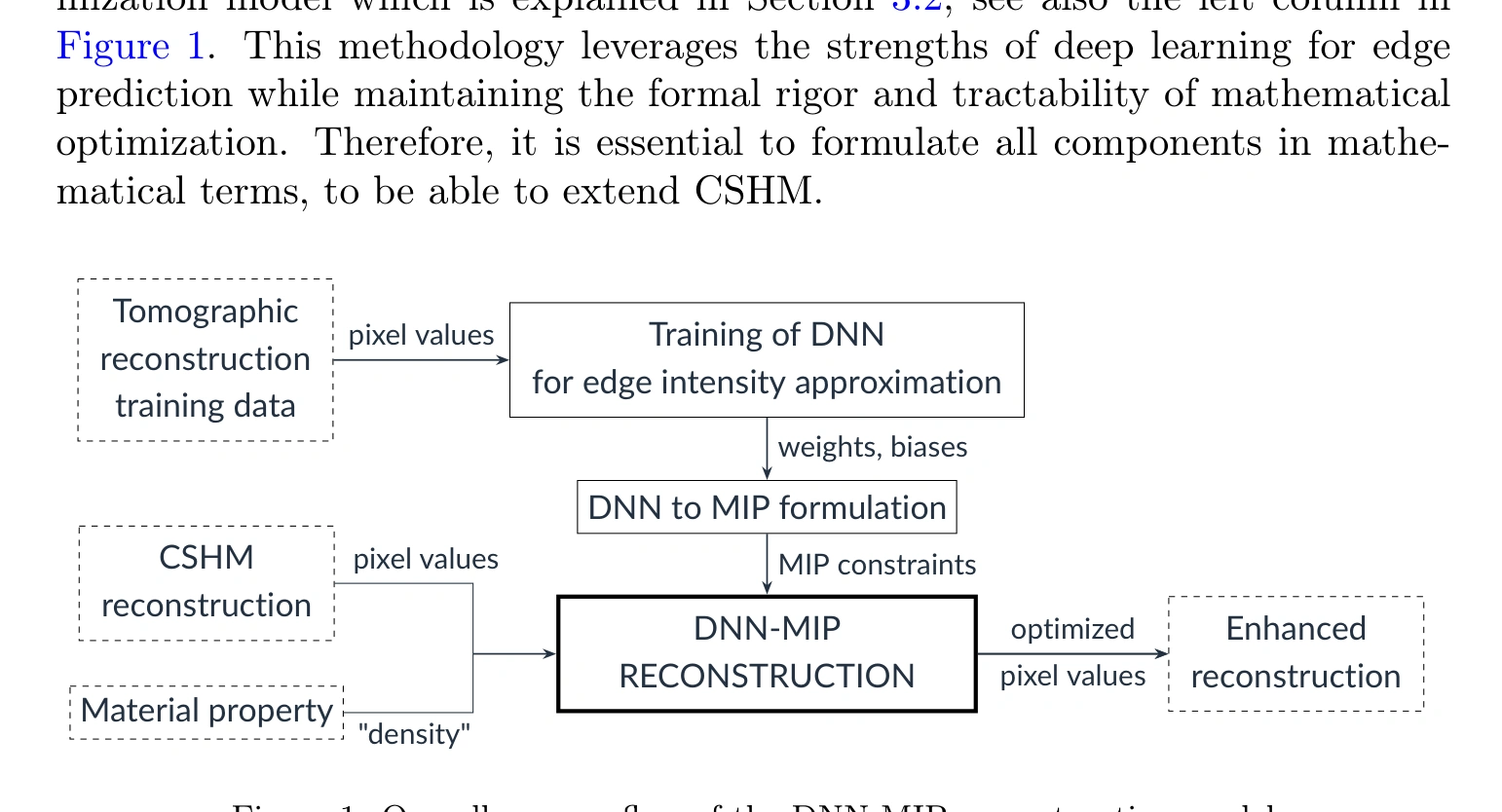
AUTHENTIC PUBLISHED FIGURE (FIGURE 1)ORIGINAL PUBLICATION SCHEMATIC

Published Figure 1: Overall process flow of the DNN-MIP reconstruction model

Published method workflow. The trained DNN approximates local edge intensity; its learned weights and biases are converted into mixed-integer constraints and integrated with the CSHM reconstruction and material-property prior. Adapted from Figure 1 in Mishra et al., Machine Learning: Science and Technology 6 (2025) 045065, CC BY 4.0 · DOI: 10.1088/2632-2153/ae25b6.

MATHEMATICAL FORMULATION

From Tomography Physics to a Learned Mixed-Integer Reconstruction Prior

A whiteboard-style mathematical derivation connecting measurement physics, compressed sensing, local neural priors, and mixed-integer patch re-optimization:

TOMOGRAPHY MODEL

R f = p

With sparse / noisy measurements:

\min_f \, \|R f - p\|_2^2

CSHM BASELINE

\operatorname{CSHM}(f) = \|R f - p\|_2^2 + \lambda \|f\|_{\mathrm{TV}} + \mu \|d\|_2^2

Balances projection fidelity with total variation regularization ( $\lambda$ ) and material density penalties ( $\mu$ ).

View published CSHM constraints↓

d_j \ge f_j - \omega, \quad d_j \ge 0 \qquad \forall \, 1 \le j \le n

f_j \le \min_{i \,:\, R_{ij} \neq 0} \frac{p_i}{R_{ij}}, \quad f_j \ge 0 \qquad \forall \, 1 \le j \le n

Where $\omega$ is estimated constant material density and $d_j$ penalizes excess intensity.

LEARNED EDGE PRIOR

\operatorname{DNN} : [0, \omega]^{3 \times 3} \longrightarrow \mathbb{R}, \qquad f^a \longmapsto y_a

3×3 local image patch → learned local edge intensity

EDGE DECISION

c_{\mathrm{edge}}(e_a, f^a) = e_a y_a + (1 - e_a)(T - y_a)

e_a = 1 → favor strong edge (

y_a > T

)

e_a = 0 → favor homogeneous patch (

y_a < T

)

DNN-MIP RE-OPTIMIZATION

c_{\mathrm{density}}(f^a) = |\omega - f^a|\,|f^a|

and

c_{\mathrm{ref}}(f^a) = \left\| f^a - \omega \frac{f_a^*}{f_{\max}} \right\|_2^2

c_{\mathrm{RO}}(e_a, f^a) = c_{\mathrm{edge}}(e_a, f^a) - \alpha \, c_{\mathrm{density}}(f^a) - \beta \, c_{\mathrm{ref}}(f^a)

\max_{e_a, \, f^a} \; c_{\mathrm{RO}}(e_a, f^a)

subject to the learned DNN / edge-decision constraints

EDGE

c_{\mathrm{edge}}

Local edge / homogeneity preference.

DENSITY

\alpha \, c_{\mathrm{density}}

Material-intensity pressure.

REFERENCE

\beta \, c_{\mathrm{ref}}

Fidelity to the CSHM reconstruction.

View ReLU-to-MIP formulation (Eq. 6–8)↓

x^k = \sigma(W^{k-1} x^{k-1} + b^{k-1}) \tag{6}

w^\top d + b = x - s, \quad x \ge 0, \quad s \ge 0 \tag{7}

z = 1 \implies x \ge 0, \quad z = 0 \implies s \ge 0 \tag{8}

$x \ge 0$ non-negative output, $s \ge 0$ slack variable, $z \in \{0, 1\}$ binary activation decision variable.

Why does α = β simplify the objective?↓

\begin{aligned} c_{\mathrm{density}}(f) + c_{\mathrm{ref}}(f) &= (\bar{u} - f) f + \|f - f^*\|_2^2 \\ &= \bar{u} f - f^2 + f^2 + (f^*)^2 - 2 f f^* \\ &= (\bar{u} - 2 f^*) f + (f^*)^2 \end{aligned}

Because $\|f^*\|_2^2$ is a constant scalar, the non-convex quadratic term $-f^2$ cancels against the convex term $+f^2$ , making the joint objective affine in $f$ .

PRIOR EXTRACTION & ARCHITECTURE DESIGN

Why a Compact Neural Network?

In conventional deep learning, larger models with millions of parameters are standard. In mixed-integer programming, every single ReLU activation introduces continuous variables and binary indicator states into the branch-and-bound tree:

COMPLEXITY ESCALATION CHAIN

Model CapacityMORE NEURONS / ReLUs↑ Expressive Power

Auxiliary VariablesMORE BINARY STATES↑ Binary Indicator Vars

MIP FormulationLARGER OPTIMIZATION MODEL↑ Linear Inequalities

Branch & BoundHIGHER SOLVER COMPLEXITYExponential Worst-Case

Architectural Trade-Off:EDGE APPROXIMATION QUALITY ↔ SOLVER TRACTABILITY

"The DNN had to be expressive enough to approximate the edge signal, but small enough to remain practical once translated into optimization constraints."

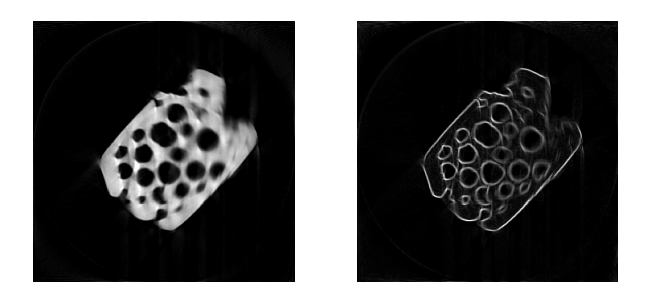
AUTHENTIC FIGURE 2 :: ZEOLITE RECONSTRUCTION VS SOBEL EDGE GRADIENT3×3 Patch Training Target

Published Figure 2: Image of a macroporous zeolite particle (left) vs. gradient image (right)

Learning the edge signal. A reconstructed zeolite slice (left) and its Sobel edge-intensity image (right), illustrating the local signal approximated by the compact neural network. Adapted from Figure 2 in Mishra et al., Machine Learning: Science and Technology 6 (2025) 045065, CC BY 4.0 · DOI: 10.1088/2632-2153/ae25b6.

SCIENTIFIC BENCHMARK RESULTS

Published Quantitative & Qualitative Results

The framework was validated on synthetic sparse projections with rigorous numerical ground truth and real physical electron tomography datasets:

PRIMARY QUANTITATIVE RESULT · FIGURE 85 Sparse Projections Benchmark

Sparse-View Interface Reconstruction

With extreme angular sparsity (only 5 projection angles), baseline compressed sensing suffers from severe boundary blurriness and streak artifacts, while DNN-MIP RO restores crisp circular interfaces:

BASELINE (d)5 Projections

CSHM Reconstruction

Relative Mean Error0.042

Bimodal Score0.974

PROPOSED METHOD (e)Sharpened Boundaries

DNN-MIP RO Reconstruction

RME (Lower is Better)0.017

BMS (Closer to 1)0.998

Sparse-view phantom reconstruction (5 projections). DNN-MIP RO reduces relative mean error (RME) from 0.042 for CSHM to 0.017 and increases bimodal score (BMS) from 0.974 to 0.998. Adapted from Figure 8 in Mishra et al., Mach. Learn.: Sci. Technol. 6 (2025) 045065, CC BY 4.0 · DOI: 10.1088/2632-2153/ae25b6.

PRIMARY EXPERIMENTAL RESULT · FIGURE 11Transmission Electron Tomography

Look at the Interface — Local Region of Interest Analysis

High-magnification inspection of local regions of interest demonstrates the complete removal of washed-out grayscale boundary transitions in favor of crisp material interfaces:

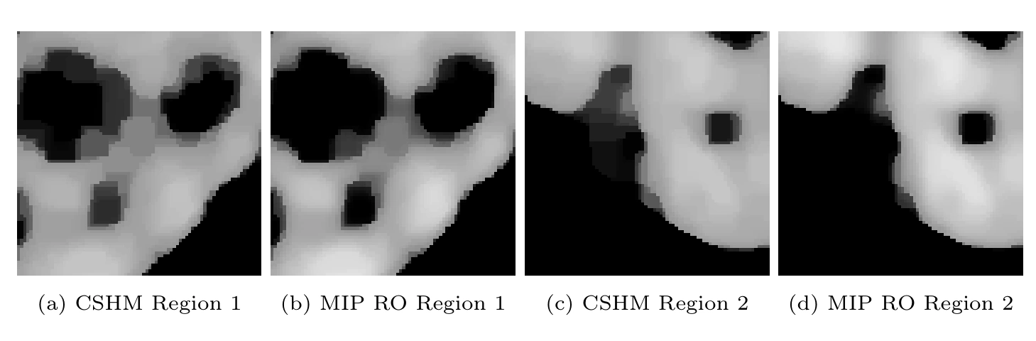
Published Figure 11: CSHM vs. MIP RO local comparison of two regions of interest for the zeolite particle

Local interface comparison (Zeolite). Cropped regions of interest demonstrate that DNN-MIP RO establishes clear boundary transitions between pore space and the zeolite framework, avoiding staircase and blur artifacts. Adapted from Figure 11 in Mishra et al., Mach. Learn.: Sci. Technol. 6 (2025) 045065, CC BY 4.0 · DOI: 10.1088/2632-2153/ae25b6.

KEY EXPERIMENTAL INSIGHT

Lowest Data Residual ≠ Always Best Physical Reconstruction

In pure mathematical simulation, minimizing projection residual ||Rf − p||² directly correlates with image fidelity. In physical experiments, raw measurements often contain non-ideal phenomena such as slight beam misalignments, contrast variations, and instrument noise.

Blindly minimizing residual against flawed measurements fits the artifacts rather than the sample. True reconstruction quality requires balancing Data Consistency against Structural / Material Homogeneity.

FULL BENCHMARK CONTEXT · 5 ALGORITHMS (FIGURE 10)SIRT · CS · TVR-DART · CSHM · DNN-MIP RO

Complete overview of the entire zeolite slice across five reconstruction paradigms:

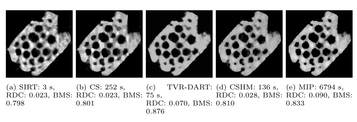
Published Figure 10: Complete benchmark across five reconstruction algorithms on experimental zeolite electron tomography

Complete 5-algorithm comparison on experimental zeolite. (a) SIRT, (b) CS, (c) TVR-DART, (d) CSHM, and (e) DNN-MIP RO. Adapted from Figure 10 in Mishra et al., Mach. Learn.: Sci. Technol. 6 (2025) 045065, CC BY 4.0 · DOI: 10.1088/2632-2153/ae25b6.

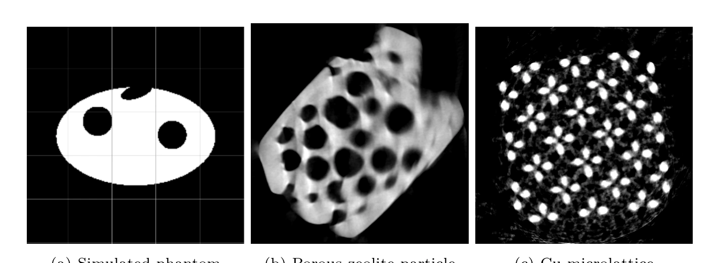
DATASET CONTEXT · FIGURE 33 Evaluation Datasets

Published Figure 3: Three different datasets used in this study: (a) simulated phantom, (b) zeolite particle, (c) Cu microlattice

(a) Simulated phantom with ground truth; (b) Porous zeolite particle; (c) Copper microlattice nano-CT. Mishra et al. (2025).

SCIENTIFIC COMPROMISES

Research Design Trade-Offs

01. Architecture SizingFormulation Size

MODEL CAPACITY ↔ SOLVER COMPLEXITY

A deeper convolutional network could learn more complex edge textures, but would introduce thousands of binary indicator variables, rendering the mixed-integer program computationally intractable.

02. Spatial DecompositionParallel Solvability

GLOBAL OPTIMIZATION ↔ LOCAL TRACTABILITY

Solving the entire 512×512 image in a single monolithic MIP is intractable. Decomposing into overlapping 3×3 patches enables parallel solves while merging ensures global boundary consistency.

03. Representation Trade-OffContinuous Relaxation

BINARIZATION ↔ GRAYSCALE FLEXIBILITY

Strict discrete binarization produces perfectly sharp boundaries but fails on transitional pores or partial-volume pixels. Continuous grayscale relaxation with material penalties preserves subtle densities.

04. Computational CostCompute Budget

RECONSTRUCTION QUALITY ↔ RUNTIME

Mixed-integer branch-and-bound optimization is significantly more compute-intensive than standard analytical filtered backprojection, trading compute time for high structural accuracy in sparse settings.

SCIENTIFIC ATTRIBUTION & COMPETENCIES

Contribution — CRediT Statement

MY DIRECT ROLE (CRediT TAXONOMY)

Standardized contributor roles as recognized by IOP Publishing:

Lead Contribution:

✓Software (algorithmic implementation, PyTorch & Gurobi integration)
✓Investigation (sparse-view experimental testing, noise sensitivity)
✓Formal Analysis (mathematical constraint formulation, error metrics)
✓Data Curation (electron tomography & nano-CT benchmark preparation)

Equal Contribution:

ConceptualizationMethodologyValidationVisualizationWriting — original draftWriting — review & editing

Co-authored with Andrea Gilch, Benjamin Apeleo Zubiri, Jan Rolfes, and Frauke Liers at Friedrich-Alexander-Universität Erlangen-Nürnberg.

WHAT THIS RESEARCH DEMONSTRATES

Key research and computational skills applied in this paper:

Neural NetworksMixed-Integer ProgrammingMathematical OptimizationTomographic ReconstructionScientific ComputingPyTorchGurobiImage / Edge AnalysisBenchmark DesignHPC / Parallel ExperimentationResearch ValidationScientific Writing

CORE SCIENTIFIC CONCLUSION

"This was not a black-box image enhancement model. We turned learned edge behavior into optimization constraints and used those constraints to improve a physically grounded reconstruction process."

The project sits at the intersection of machine learning and mathematical optimization: learn a useful local prior from data, translate that learned model into explicit optimization constraints, and let the solver balance that prior against reconstruction fidelity and material structure.